Solving your first problem with Bempp

This page gives and overview of Bempp, and guides you through solving your first Laplace problem.

Before following this tutorial, you will need to install Bempp. Once you have Bempp installed, open a Jupyter notebook or a Python or IPython terminal and you are ready to begin.

Importing Bempp

First, you need to import Bempp.

Bempp is split into two parts: bempp.api and bempp.core: bempp.api contains the library’s Python functionality and bempp.core contains the interfaces to the fast OpenCL (or C++ if you’re using the previous version) computational kernel. As a user you (almost certainly) want to begin by importing bempp.api:

import bempp.api

Generating a grid

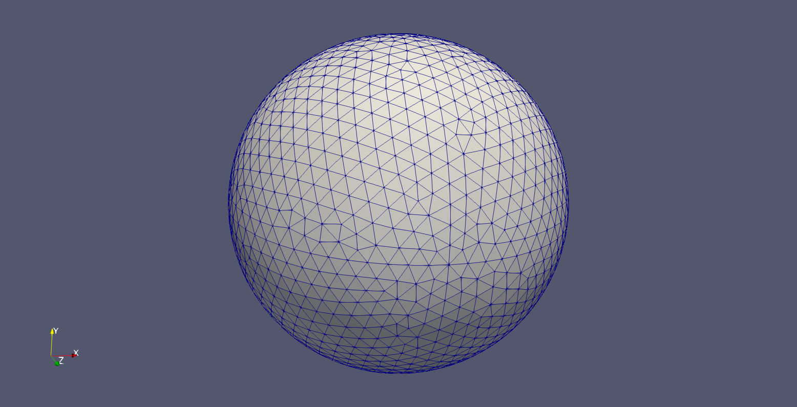
Bempp solves discretised problems on grids (or meshes) of triangular cells. Before solving your problem, you must create or import your grid.

In this example, we will use a sphere. The following code snippet will create your grid.

grid = bempp.api.shapes.sphere(h=0.1)
grid.plot()

If you are using a Jupyter notebook, then the second line in this snippet will visualise your grid using plotly. If you are not using a notebook, you will need to change the plotting backend in order to visualise your grid. The following code, for example, will visualise your grid using Paraview.

bempp.api.PLOT_BACKEND = "paraview"
grid.plot()

If all is well, you will now have created and visulaised your grid.

More information about grids can be found in the grids tutorial.

Defining a function space

Next, you need to build a function space on the grid. In this case, we use a space of piecewise constant polynomials, or order 0 discontinuous polynomials (DP).

The following code snippet will create this function space.

space = bempp.api.function_space(grid, "DP", 0)

Building boundary operators

Next, you can build boundary operators using the spaces you have defined. In this example, we construct a Laplace single layer boundary operator.

This operator can be defined using the following Python snippet.

slp = bempp.api.operators.boundary.laplace.single_layer(space, space, space)

Constructing a grid function

Next, we construct a grid function containing your right-hand-side data. In this example, we use a Python function to construct our grid function. As our function is real-valued, we must use the @bempp.api.real_callable decorator so that Bempp can use the correct number types in its compiled code.

@bempp.api.real_callable
def f(x, n, domain_index, result):
    result[0] = x[0] + 1


rhs = bempp.api.GridFunction(space, fun=f)

Solving

Now that you have constructed all the necessary objects, you are ready to solve the discretised problem. In this case, we use GMRES to solve the problem.

sol, info = bempp.api.linalg.gmres(slp, rhs)

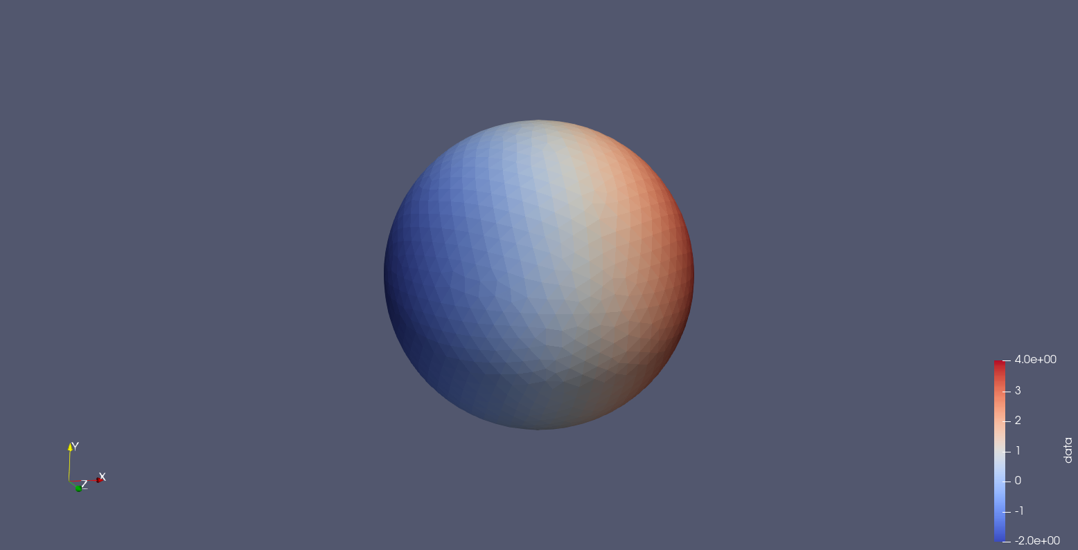
Finally, you can visualise your solution:

sol.plot()

What’s next?

A list of further documentation and tutorials can be found on the documentation page.